Delay Coordinate Embeddings with Python
In this article, I will describe what a delay coordinate embedding is and how to interpret one with the help of visuals generated by a python script given at the bottom.
What is a Delay Coordinate Embedding?
A delay coordinate embedding is a form of state space reconstruction, where one dimensional sensor data, a sampling of the system state, is reconstructed in a higher dimensional space, with lag. This means that each value of the time series, x(t), is plotted against its value at x(t-T), x(t-2T), … in a higher dimensional embedding space. The generated space can serve as a useful model of a system’s state change dynamics, especially useful in chaotic complex systems, in which, the time series would be otherwise uninterpretable. This idea is largely based on Takens’s Theorem, a delay embedding theorem, where Floris Takens lays out the conditions under which a chaotic dynamical system can be reconstructed from a sequence of observations of the system’s state, rendering a topological diffeomorphism of its true dynamics[1].
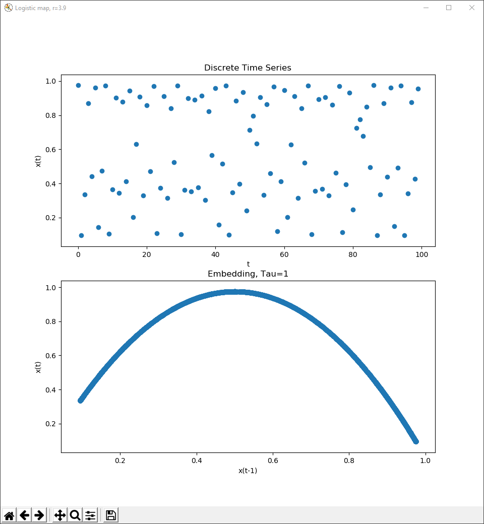
The Logistic map with r=3.9, under chaos, time series and delay coordinate embedding, download data.
How to Interpret and Why They’re Useful
To start, a dynamical system is a system which has a state, x, determined by an evolution rule that acts on the system’s previous state – x(t+1) = f(x(t)), otherwise written as xdot = f(x)[2]. Many times, these systems settle onto fixed values or follow periodic orbits, both of which are very easy to interpret when presented as a time series, but, it is possible that these systems are shown to be very complex or even chaotic and seemingly randomly change over time.
The Lorenz system is a fantastic example of a dynamical system that is far too complex to understand just as a time series, demonstrated in an interesting article here, but, is easily understood as a delay coordinate embedding, as shown here and here.
A great example of a chaotic system, is the Logistic map at r > 3.5. The Logistic map is a family of functions, originally created by Robert May to model discrete population dynamics in his paper Bifurcations and Dynamic Complexity in Simple Ecological Models. The system’s state represents the percentage of population capacity occupied, and is governed by the rule, xdot = rx(1-x), where r is a hyper parameter, that does not change during the evolution of the system, representing the reproduction rate of a given species within the interval [0, 4][3]. At r values less than one, the system stays at a fixed point, 0, because the population dies off due to insufficient reproduction. Between r = 1 and 3, the fixed point at which the population stabilizes grows with r because the die off rate keeps up with reproduction. From r = 3 to roughly 3.4, the system is in an orbit, in which the state, the population, alternates between two values. From r = 3.4 to 3.5 the orbit has a period doubling bifurcation multiple times, where the number of points in the orbit doubles. Finally, at a little more than r=3.5 the system becomes chaotic, under which the population changes at what visually amounts to randomness, but is actually an orbit that is very difficult to interpret as a time series. More on the bifurcations of the Logistic map on my github and this blog post by Geoff Boeing.
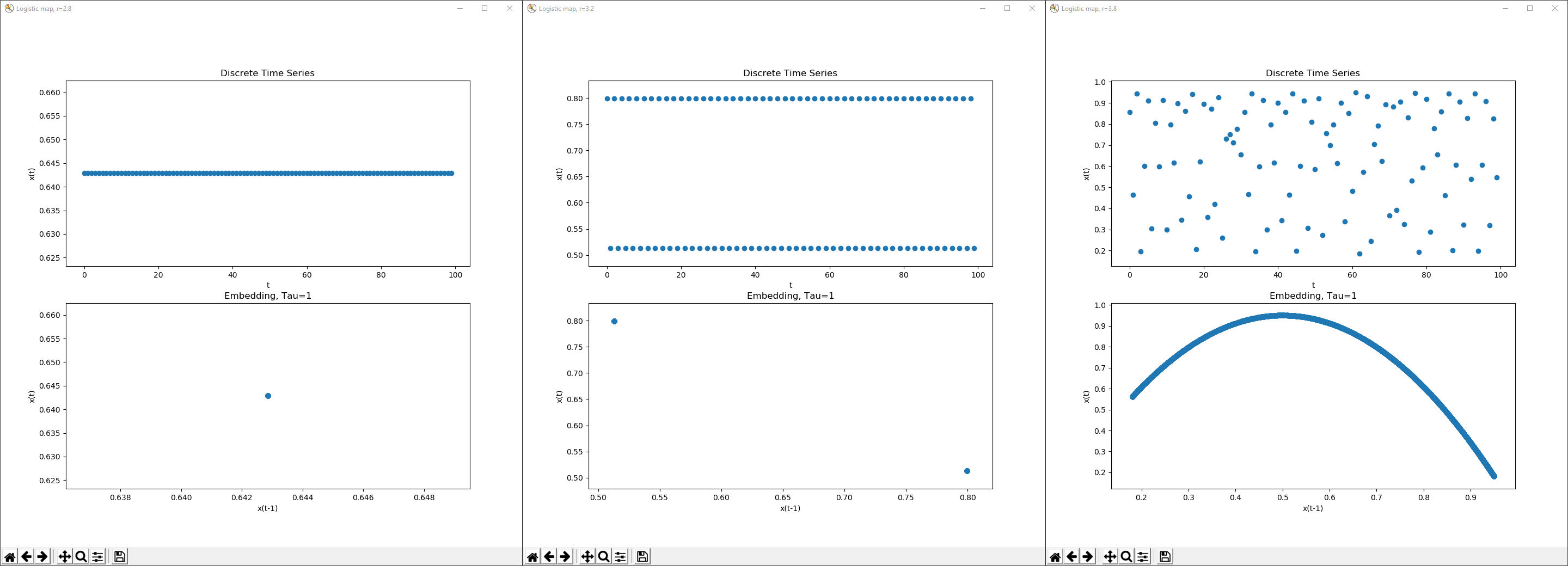
The time series(top) and delay coordinate embeddings(bottom) of the Logistic map with r=2.8, 3.2 and 3.8, Tau=1, showing increasing amounts of complexity. Each piece of data was taken after 100 iterations, giving the systems time to stabilize. It should be noted that while the time series are shown with 100 iterations, the delay coordinate embeddings use 5000.
Here, the Logistic map is shown first with a fixed point, then as a two point periodic orbit and finally under chaos at r = 3.8. Even though the time series begins to appear random, the delay coordinate embedding depicts the system as following very clear rules. The embedding has a value for Tau, the delay parameter, equal to 1, and in the axes of this plot are respectively, x(t-1) and x(t). For example, a point at (.5, 1.0) means, when the system reaches the state .5, after Tau time, the system will hit state 1.0. Thus, making delay coordinate embedding incredibly useful for prediction.
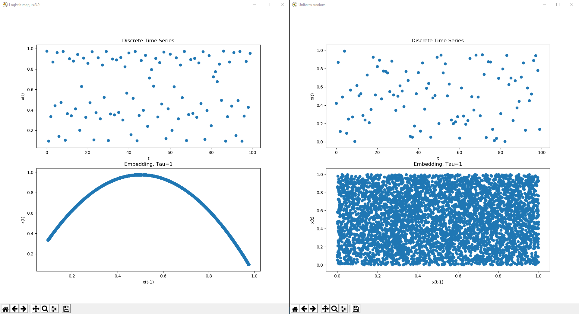
A chaotic time series and delay coordinate embedding from the logistic map at r=3.9 in constrast to uniform random data.
Parameters
Tau is a measure of time, in which the axes of the reconstruction will be generated – x(t), x(t-Tau), x(t-2Tau), and so on. As shown above, a Tau of 1 unit of time, would plot the state, x(t), against its prior self, one time step earlier at x(t-1). This value dictates how granular the values of the system’s history are shown. Thus, a large Tau will show the connections between states very far in the past, to those far in the future, and therefore the potential to make the reconstruction very complex.
The choice of embedding dimension dictates how many axes will be used in reconstruction space, thus, how much of the system’s history is shown. The dimensionality must be high enough to provide relevant information, while small enough to easily comprehend. A high embedding dimension will create a rich history of the systems state over time, though, it will take a proportional amount of effort to interpret.
Information and Formal methods for choosing these parameters can be found at the bottom of this article, but, for many simple systems they can be brute forced.
Python Code
"""
Python 3, requires the library matplotlib and a csv file with evenly sampled data.
"""
FILENAME = 'henon_a14b03.csv'
COLUMN = 0       ## Which column of csv file to use, 0 means leftmost.
POINTS = -1      ## Number of points to use, more can be slower to render.
                 ## -1 if all(but last).

E_DIMENSION = 2  ## Number of dimensions in embedding space -- 2 or 3.
TAU = 1          ## Delay, integer


import csv

import matplotlib.pyplot as plt  ## pip install matplotlib
from mpl_toolkits.mplot3d import Axes3D


if __name__ == '__main__':
    ## Read Data
    with open(FILENAME, 'r') as file:
        time_series = [float(row[COLUMN]) for row in csv.reader(file)][:POINTS]

    ## Process Data
    if E_DIMENSION == 2:
        delay_coordinates = [
            time_series[:-TAU if TAU else len(time_series)],    # t-T
            time_series[TAU:]                                   # t
            ]
    elif E_DIMENSION == 3:
        delay_coordinates = [
            time_series[TAU:-TAU if TAU else len(time_series)], # t-T
            time_series[2 * TAU:],                              # t
            time_series[:-2 * TAU if TAU else len(time_series)] # t-2T
            ]
    else:
        raise ValueError(f"Invalid Embedding Dimension, '{E_DIMENSION}' not in [2, 3]!")

    ## Visualize Embedding
    fig = plt.figure()

    # Raw time series data
    ax = fig.add_subplot(211)
    ax.scatter(range(len(time_series[:100])), time_series[:100])
    ax.set_title('Discrete Time Series')
    ax.set_xlabel('t')
    ax.set_ylabel('x(t)')

    # Reconstruction space
    ax = fig.add_subplot(212, projection='3d' if E_DIMENSION == 3 else None)
    ax.scatter(*delay_coordinates)
    ax.set_title(f'Embedding, Tau={TAU}')
    ax.set_xlabel(f'x(t-{TAU})')
    ax.set_ylabel('x(t)')
    if E_DIMENSION == 3:
        ax.set_zlabel(f'x(t-{2*TAU})')

    plt.show()
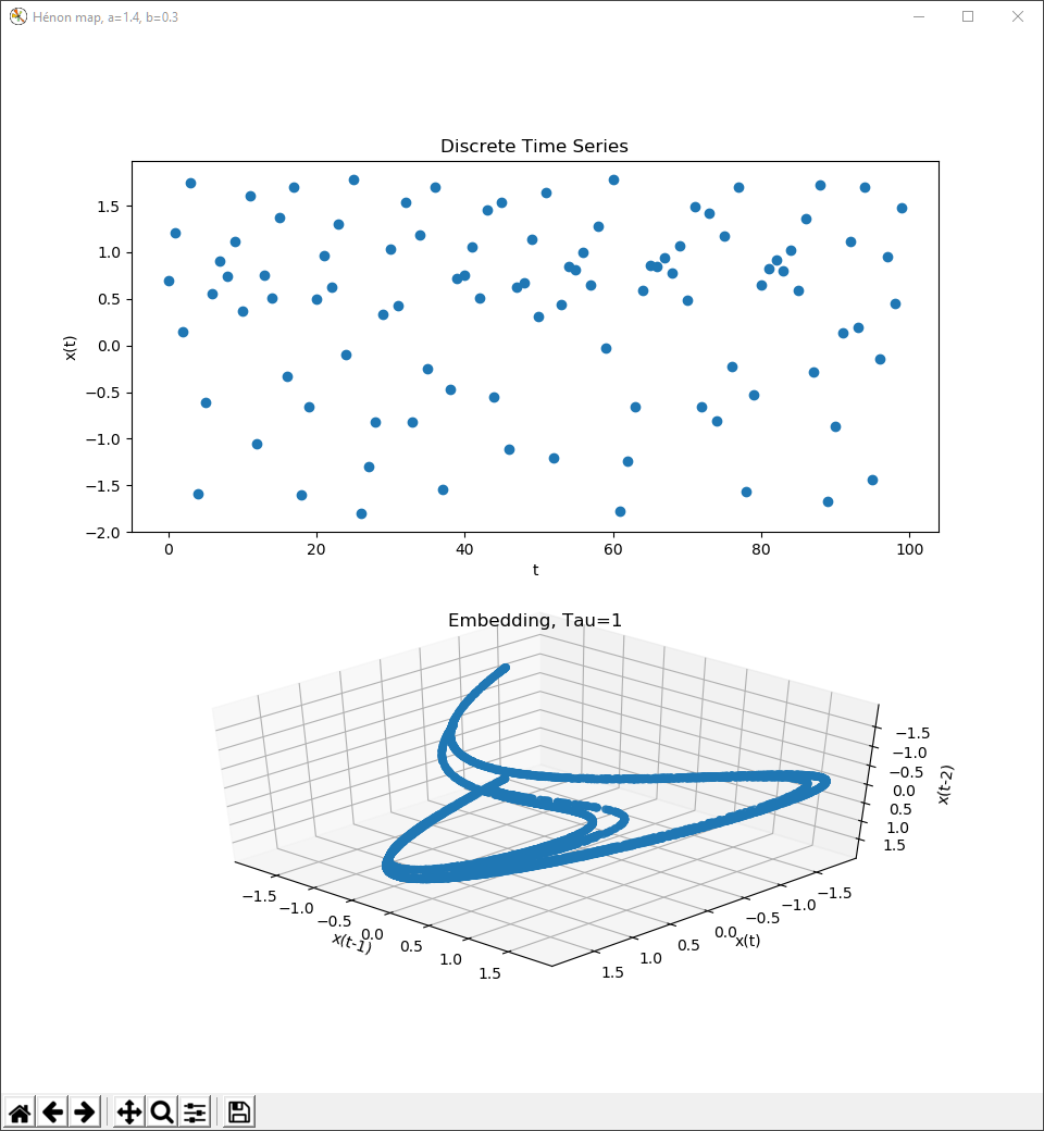
This is the x value of the Hénon map, at a=1.4 and b=0.3, time series and delay coordinate embedding.
Finding Useful Parameters
A lag value and embedding dimension need to be chosen specifically for the system, poorly chosen parameters can render uninterpretable or topologically incorrect visualizations. Methods have been devised to find these parameters and can even be automated.
Complexity Explorer video on methods of finding Tau
Complexity Explorer video on methods of finding an Embedding Dimension
A lower tau is typically best, for simplicity, and a coordinate embedding in 2 or 3 dimensions is optimal for visualization.
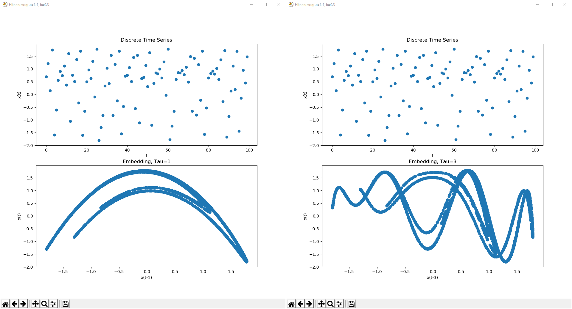
An example of the Hénon map at a=1.4 and b=0.3, with delay coordinate embeddings of Tau=1 and Tau=3.
Sources
More Reading
Chapter on Delay Coordinate Embedding
Seminar Presentation on Takens Theorem
Scholarpedia: Attractor Reconstruction
Eric Weeks: Adventures in Chaotic Time Series Analysis